
Finding Backcountry Campsites with CalTopo, OpenStreetMap, and R
Published:
Like many people, I’ve been spending more time outdoors during this pandemic. While this means daily walks in my neighborhood, it also means getting out into the wilderness and sleeping in a tent when I can. Although outdoor recreation is one of the safer ways to entertain yourself these days, it’s not without its own concerns. The difficulty of safely getting to trailheads means that while I’m backpacking more than usual, it’s still not as often as I’d like.
That means I’m spending a decent chunk of time thinking about and planning future trips. At some point in the process of doing this, I realized that I could use the GIS skills from my day job to help make planning future trips more efficient. In this post I walk through how you can use GIS tools in R to help with some of the route planning for a multiday backpacking trip. Specifically, how you can use open source spatial data on geography and transportation infrastructure to identify potential campsites along a hiking trail.
This was largely an exercise in seeing how I could apply GIS skills I’ve learned in the study of political violence to small-scale GPS navigation. I haven’t had the opportunity to hit the trail and test out any of the assumptions I use in this process yet, so you should view this post as more of a (loose) method than concrete suggestions. For a short and simple point-to-point hike with only one route, there’s really no need to engage in this level of GIS analysis. I’ve kept things simple to make them easier to follow, but this approach could actually be useful and save some time when planning a longer trip with many potential routes.
Backcountry camping
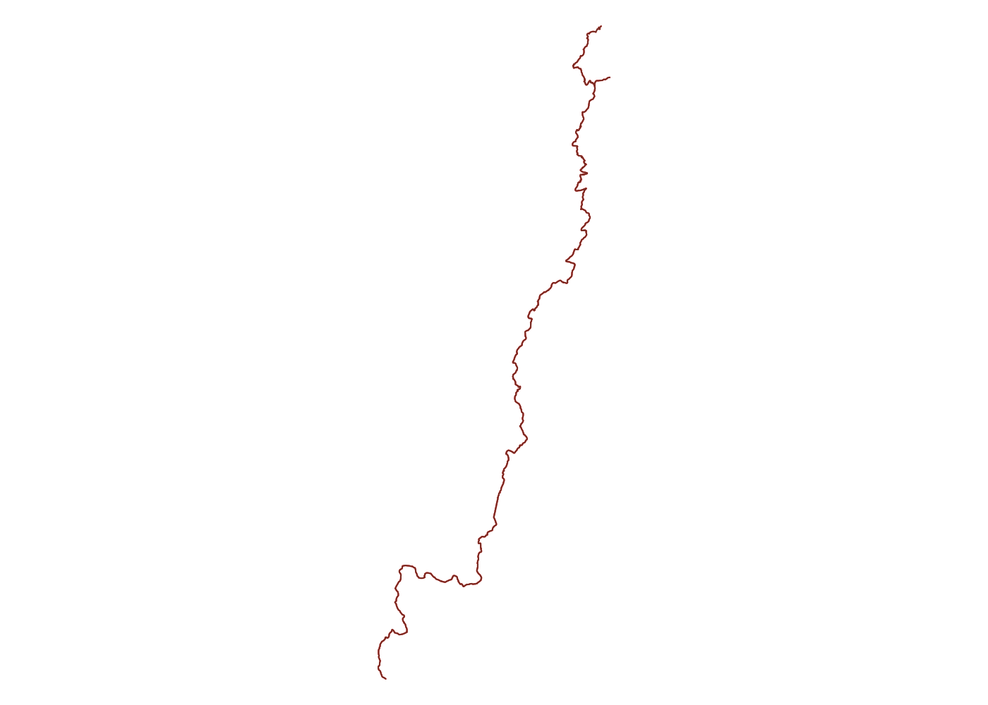
At some point in the future, I want to hike the Uwharrie Trail in Uwharrie National Forest in central North Carolina, near where I went to grad school. As I think about this (probably far off) trip, I’ve been using CalTopo to plan my route.
If you spend any amount of time in the outdoors, you should know about CalTopo. CalTopo is a website that lets you plan routes (hiking, skiing, rafting, etc.) on top of super high resolution topographic maps. You can then turn your smartphone into a full-featured GPS and use it to follow those routes (CalTopo offes a mobile app, as does Gaia GPS, both for about $20 a year). While the Uwharrie Trail is a pretty straightforward hike, I’ve been using this as an excuse to try and apply my GIS skills in a new context.
CalTopo is great, but it’s very point and click. I like doing things programmatically when I can, so that means it’s time to grab some of the open source data that CalTopo uses so we can play around with it in R. The base map in CalTopo is called MapBuilder Topo, and uses OpenStreetMap data as its starting point, so let’s start there.
Disclaimer
This guide is intended to show how to identify potential backcountry campsites on public land where dispersed camping is permitted. If you are backpacking in an area with designated, maintained backcountry campsites, you should use them. Dispersed camping is typically permitted in less-traveled areas where the impact of campers is better minimized by diffusing it rather than concentrating it into a handful of designated sites.1
Always check regulations for any land you plan to camp on to see if there are specific requirements for site selection or areas where camping is prohibited. Picking an actual campsite requires identifying areas where your saftey will be maximized and the longterm impact of your stay will be minimized. See this guide for the basics and this series for a slightly more hardcore set of principles to follow. And remember, never go into the wilderness without telling someone where you’re going and when you should be back.
Getting the data
OpenStreetMap (OSM) is an open source map of the entire globe; think of it as a hybrid of Google Maps and Wikipedia. OSM is designed so that anyone can easily add to or edit it. Setting aside the normative value of this perspective, this is helpful for us because it means that OSM is transparent. We can use the excellent osmdata R package to query OSM via the [Overpass API], and we can use OSM itself via the OSM website to learn the various parameters we’ll use to query OSM.
Trails
The getting started vignette covers much of the basics of using osmdata. The key functions are osmdata::opq(), which builds a query to the Overpass API, and osmdata::add_osm_feature(), which requests specific features. OSM classifies features using key-value pairs, and we can use the OSM website to figure out just which pairs we need. Navigate to an area of interest, right-click on the feature of interest, and then select “query features.”
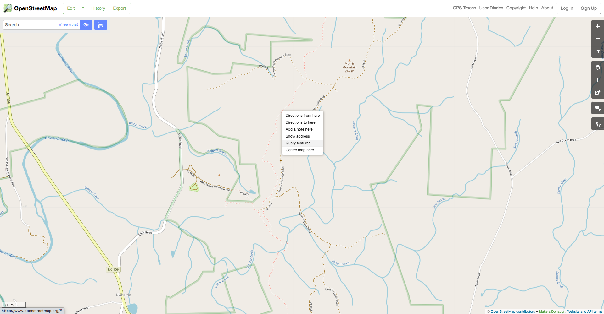
Next, select the desired feature in the dialog on the left of the screen. In this case, select the “Relation” rather than the “Path” because the path will only include one segment of the trail while the relation will include its entire length.
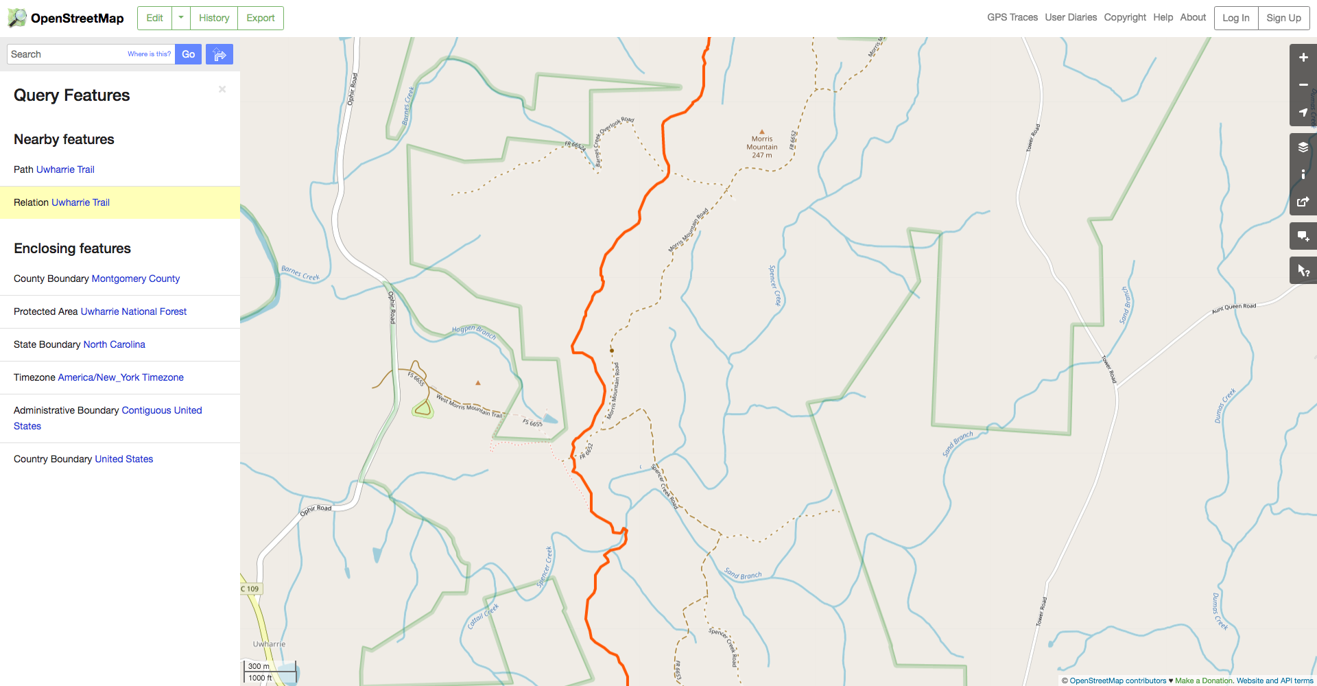
We can see here that the Uwharrie Trail relation has type=hiking, so that’s the key-value pair wew’ll have to specify in our query.

Make sure to use the bbox argument to osmdata::opq(), otherwise you’ll request every hiking trail in the world! You can manually specify the four edges of a bounding box to search in, or you can use the osmdata::getbb() function to get it automatically using the Nominatim geocoder.
library(tidyverse)
library(sf)
library(osmdata)

## get hiking routes in Uwharrie National Forest
unf_trails <- opq(bbox = getbb('uwharrie national forest usa')) %>%
  add_osm_feature(key = 'route', value = 'hiking') %>%
  osmdata_sf()
Notice that we use the osmdata::osmdata_sf() function to convert the resulting object for use with the sf R package. Let’s inspect the resulting object of class osmdata_sf.
## inspect
unf_trails
## Object of class 'osmdata' with:
##                  $bbox : 35.3951403,-80.0236608,35.4351403,-79.9836608
##         $overpass_call : The call submitted to the overpass API
##                  $meta : metadata including timestamp and version numbers
##            $osm_points : 'sf' Simple Features Collection with 3341 points
##             $osm_lines : 'sf' Simple Features Collection with 26 linestrings
##          $osm_polygons : 'sf' Simple Features Collection with 0 polygons
##        $osm_multilines : 'sf' Simple Features Collection with 1 multilinestrings
##     $osm_multipolygons : NULL
We can see that the unf_trails object includes points, lines, polygons, multilines, and multipolygons. We want to use the lines since that will include any short trail segments that aren’t part of a larger trail. We can easily plot the trails using this object.
## plot
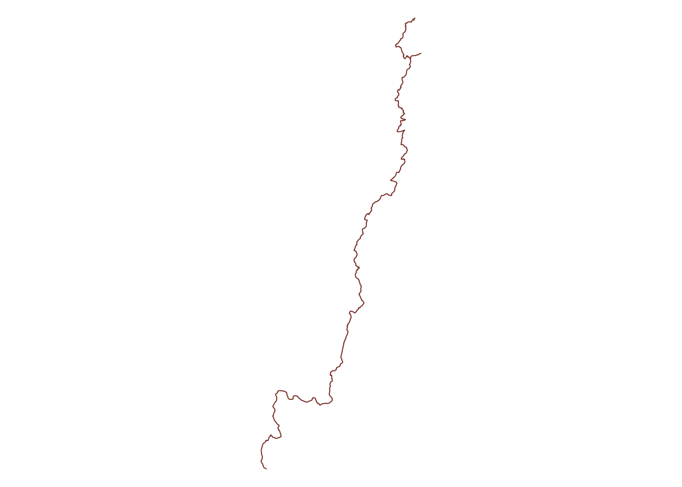
plot(unf_trails$osm_lines$geometry, col = 'coral4')
Don’t get lost
Let’s do some quick sanity checks. First, Wikipedia tells us the trail should be about 20 miles. We can use the sf::st_length() function to measure the length of each trail segment, and the sf::st_union() function to combine all segments. We’ll get our answer in meters, which as a metric-deprived American, won’t be all that helpful to me. To get around this, we can use the `units::st_units() function to convert from meters to miles.
## measure total trail length
st_union(unf_trails$osm_lines$geometry) %>% # combine all segments.
  st_length() %>% # measure length
  units::set_units(mi) # convert to miles
## 28.26457 [mi]
While that’s initially concerning, a closer reading of the Wikipedia article for the trail reveals that it was originally 40 miles long, so OSM likely includes some of the Northern section of the trail beyond what’s officially recognized today.
We should also plot the bounding box that osmdata::getbb() ends up generating to ensure we’re not missing any part of the trail. We can do this with the OpenStreetMap [R package](https://cran.r-project.org/package=OpenStreetMap. Here we unfortunately need to manually specify the bounding box as a series of two vectors with the latitude and longitude coordinate of the upper-left and lower-right of the box. OpenStreetMap::openmap() uses (latitude, longitude) pairs, not (longitude, latitude) pairs as is more common in GIS, i.e., (y, x) not (x, y), so be sure to include them in that order.[^lat-long]{markdown} OpenStreetMap::openproj() also requires a projection argument, so I use sf::st_crs(4326)$proj4string to generate one automatically, ensuring I don’t introduce a type somewhere by accident.
[^lat-long]:{markdown} I spent 20 minutes not understanding why I couldn’t get this to work before I finally read the documenation. Don’t be like me, folks.
library(OpenStreetMap)

## get bounding box
unf_bb <- getbb('uwharrie national forest usa')

## get OSM tiles
unf_tile <- openmap(c(unf_bb[2,1],  # lat
                      unf_bb[1,1]), # long
                    c(unf_bb[2,2],  # lat
                      unf_bb[1,2]), # long
                    type = 'osm', mergeTiles = T)

## project map tiles and plot (OSM comes in Mercator...)
plot(openproj(unf_tile), projection = st_crs(4326)$proj4string)

## plot trails
plot(unf_trails$osm_lines$geometry, add = T, col = 'coral4')
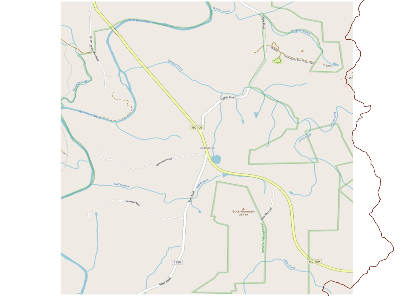
Uh oh. We can see that we’re only getting a small portion of the total trail and that it trails (heh) off the map on three sides. That’s not great, so let’s fix it. We can start by looking up Uwharrie National Forest itself on the OSM website. This gives us the boundaries of the official forest land in orange.
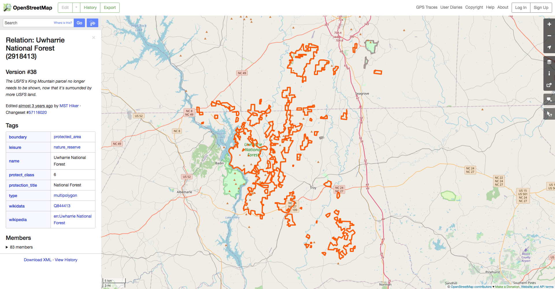
We can see from the dialog on the left that the forest’s OSM ID is 2918413, so we can use the osmdata::opq_osm_id() function to get the polygons for the forest’s boundaries. Let’s grab the forest boundaries and plot them, along with the bounding box they imply and the bounding box that resulted from osmdata::getbb() (in red) for comparison.
## get Uwharrie National Forest Boundaries
unf <- opq_osm_id(type = 'relation', id = 2918413) %>%
  osmdata_sf()

## plot Uwharrie National Forest polygons
plot(unf$osm_multipolygons$geometry, col = 'lightgreen', border = NA, bty = 'n')

## construct line for original bounding box
plot(st_multilinestring(list(matrix(c(unf_bb[1, 1], unf_bb[2, 1],
                                      unf_bb[1, 1], unf_bb[2, 2],
                                      unf_bb[1, 2], unf_bb[2, 2],
                                      unf_bb[1, 2], unf_bb[2, 1],
                                      unf_bb[1, 1], unf_bb[2, 1]),
                                      ncol = 2, byrow = T))),
     add = T, col = 'red')

## plot bounding box for Uwharrie National Forest polygons
plot(st_as_sfc(st_bbox(unf$osm_multipolygons)), add = T)

## plot trails
plot(unf_trails$osm_lines$geometry, add = T, col = 'coral4')
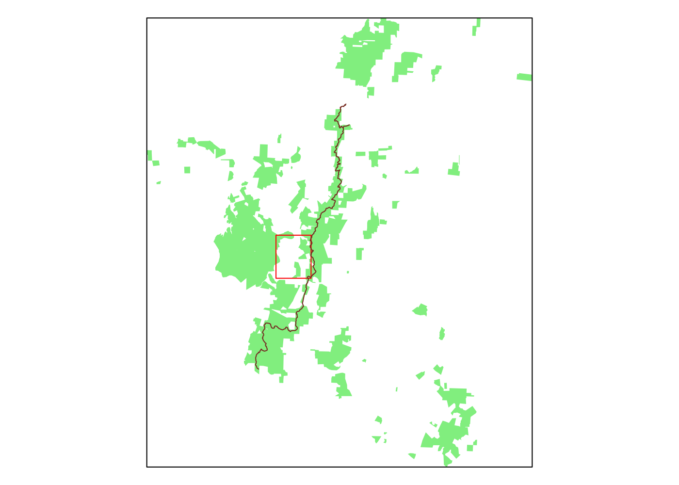
Wow, we were missing a lot before. Let’s use the bounding box for the entire forest as our new bounding box. First, we plot OSM using this new bounding box. st_bbox() yields a vector of four numbers, rather than the matrix that osmdata::getbb() produces, so we need to work around this and specify the top-left and bottom-right corners of our new, bigger bounding box.
## get OSM tile for Uwharrie National Forest polygons
unf_full_tile <- openmap(c(st_bbox(unf$osm_multipolygons)[4],  # lat
                           st_bbox(unf$osm_multipolygons)[1]), # long
                         c(st_bbox(unf$osm_multipolygons)[2],  # lat
                           st_bbox(unf$osm_multipolygons)[3]), # long
                         type = 'osm', mergeTiles = T)

## project and plot OSM tile
plot(openproj(unf_full_tile), projection = st_crs(4326)$proj4string)

## plot trails
plot(unf_trails$osm_lines$geometry, add = T, col = 'coral4')
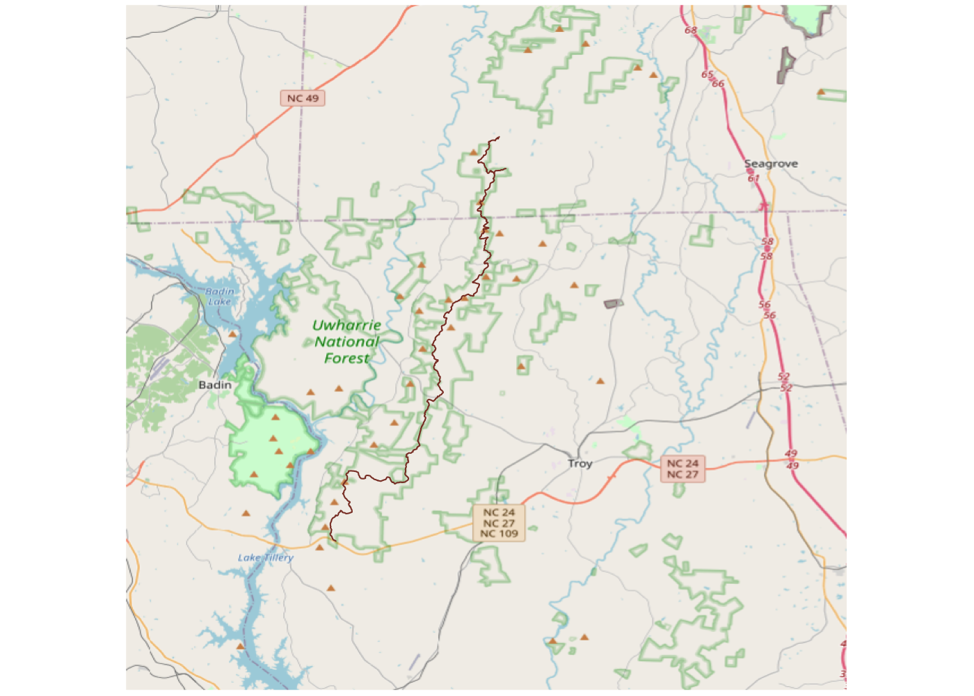
That’s much better! We’re getting a lot of area beyond the trail, but it’s easy to filter that out later so it’s better to grab too much than too little.
The whole trail
Now we can go back and grab all hiking trails in Uwharrie National Forest using our new bounding box. osmdata::opq() expects a bounding box in a certain format, so let’s inspect it to see what we’re working with and what we need to reshape the output of sf::st_bbox(unf$osm_multipolygons) into:
## bbox format osmdata::opq() expects
unf_bb
##         min       max
## x -80.02366 -79.98366
## y  35.39514  35.43514
## rearrange sf::st_bbox() output
matrix(st_bbox(unf$osm_multipolygons), ncol = 2,
       dimnames = list(c('x', 'y'), c('min', 'max')))
##         min       max
## x -80.17085 -79.73170
## y  35.21987  35.63684
Note that I’m specifying row and column names when creating the new bounding box. Without them, osmdata::opq() will fail! We can now plug this new bounding box object into osmdata::opq() and get all hiking routes in the forest.
## get hiking trails in all of Uwharrie National Forest
unf_trails_full <- opq(bbox = matrix(st_bbox(unf$osm_multipolygons), ncol = 2,
                                     dimnames = list(c('x', 'y'), c('min', 'max')))) %>%
  add_osm_feature(key = 'route', value = 'hiking') %>%
  osmdata_sf()

## plot
plot(unf_trails_full$osm_lines$geometry, col = 'coral4')
Now we’re getting a bunch of trails across the Pee Dee River in Morrow Mountain State Park. Again it’s easy to drop these extra trails later, so for the moment, more complete is better than less complete. These data come from OpenStreetMap, so they also include lots of usuable data. Let’s take a look at the fields included in our lines:
## inspect
glimpse(unf_trails_full$osm_lines)
## Rows: 106
## Columns: 37
## $ osm_id            <chr> "32024414", "216945232", "216945234", "216945241", …
## $ name              <chr> "Uwharrie Trail", "Mountain Loop Trail", "Mountain …
## $ alt_name          <chr> "Uwharrie National Recreation Trail", NA, NA, NA, N…
## $ bicycle           <chr> "no", "no", "no", "no", "no", "no", "no", "no", "no…
## $ bridge            <chr> NA, NA, "yes", "yes", NA, NA, "boardwalk", NA, NA, …
## $ construction      <chr> NA, NA, NA, NA, NA, NA, NA, NA, NA, NA, NA, NA, NA,…
## $ dog               <chr> NA, "leashed", "leashed", "leashed", "leashed", NA,…
## $ foot              <chr> "designated", "designated", "designated", "designat…
## $ footway           <chr> NA, NA, NA, NA, NA, NA, NA, NA, NA, NA, NA, NA, NA,…
## $ highway           <chr> "path", "path", "path", "path", "path", "path", "pa…
## $ horse             <chr> NA, "no", "no", "no", "no", "no", NA, NA, NA, NA, "…
## $ lanes             <chr> NA, NA, NA, NA, NA, NA, NA, NA, NA, NA, NA, NA, NA,…
## $ layer             <chr> NA, NA, "1", "1", NA, NA, "1", NA, NA, NA, NA, NA, …
## $ motor_vehicle     <chr> NA, "no", "no", "no", "no", "no", NA, NA, NA, NA, "…
## $ name_1            <chr> NA, NA, NA, NA, NA, NA, NA, NA, NA, NA, NA, NA, NA,…
## $ oneway            <chr> NA, NA, NA, NA, NA, NA, NA, NA, NA, NA, NA, NA, NA,…
## $ rcn_ref           <chr> NA, NA, NA, NA, NA, NA, NA, NA, NA, NA, NA, NA, NA,…
## $ sac_scale         <chr> NA, "mountain_hiking", "mountain_hiking", "mountain…
## $ service           <chr> NA, NA, NA, NA, NA, NA, NA, NA, NA, NA, NA, "parkin…
## $ smoothness        <chr> NA, "bad", "good", "good", "bad", NA, NA, NA, NA, N…
## $ source            <chr> NA, NA, NA, NA, NA, "GPS_2009", "GPS_2009", "GPS_20…
## $ surface           <chr> "dirt", "ground", "wood", "wood", "ground", "ground…
## $ symbol            <chr> NA, NA, NA, NA, NA, NA, NA, NA, NA, NA, NA, NA, "wh…
## $ tiger.cfcc        <chr> NA, NA, NA, NA, NA, NA, NA, NA, NA, NA, NA, NA, NA,…
## $ tiger.county      <chr> NA, NA, NA, NA, NA, NA, NA, NA, NA, NA, NA, NA, NA,…
## $ tiger.name_base   <chr> NA, NA, NA, NA, NA, NA, NA, NA, NA, NA, NA, NA, NA,…
## $ tiger.name_base_1 <chr> NA, NA, NA, NA, NA, NA, NA, NA, NA, NA, NA, NA, NA,…
## $ tiger.name_type   <chr> NA, NA, NA, NA, NA, NA, NA, NA, NA, NA, NA, NA, NA,…
## $ tiger.reviewed    <chr> NA, NA, NA, NA, NA, NA, NA, NA, NA, NA, NA, NA, NA,…
## $ tiger.zip_left    <chr> NA, NA, NA, NA, NA, NA, NA, NA, NA, NA, NA, NA, NA,…
## $ tiger.zip_left_1  <chr> NA, NA, NA, NA, NA, NA, NA, NA, NA, NA, NA, NA, NA,…
## $ tiger.zip_right   <chr> NA, NA, NA, NA, NA, NA, NA, NA, NA, NA, NA, NA, NA,…
## $ tiger.zip_right_1 <chr> NA, NA, NA, NA, NA, NA, NA, NA, NA, NA, NA, NA, NA,…
## $ tracktype         <chr> NA, NA, NA, NA, NA, NA, NA, NA, NA, NA, NA, NA, NA,…
## $ trail_visibility  <chr> NA, "excellent", "excellent", "excellent", "excelle…
## $ wheelchair        <chr> NA, "no", "no", "no", "no", NA, NA, NA, NA, NA, "no…
## $ geometry          <LINESTRING [°]> LINESTRING (-80.0435 35.310..., LINESTRI…
We can use the “name” field to subset the data. If you were considering some parallel or spur trails, you could use sf::st_filter() in combination with `sf::st_is_within_distance() to instead just grab trails near your primary trail.
## extract OSM lines and filter
ut <- unf_trails_full$osm_lines %>% filter(name == 'Uwharrie Trail')
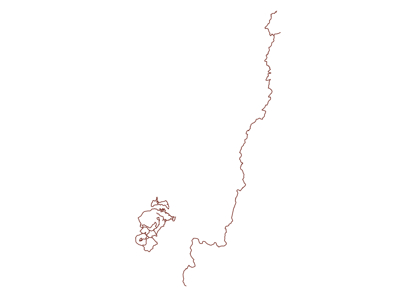
Now we’ve gotten the Uwharrie Trail twice. Once using a smaller bounding box and once using a larger one. We can plot them both and see if there were any segments the intial query missed
## plot
plot(ut$geometry, col = 'red')
plot(unf_trails$osm_lines$geometry, add = T, col = 'coral4')
Luckily the initial query still picked up every segment, but that won’t always be the case if you start with an inaccurate initial bounding box. If the entire Uwharrie Trail wasn’t collected into a relation, we might have missed large chunks of it on either end. Now we can use the bounding box for the Uwharrie Trail to capture any other features we care about nearby.
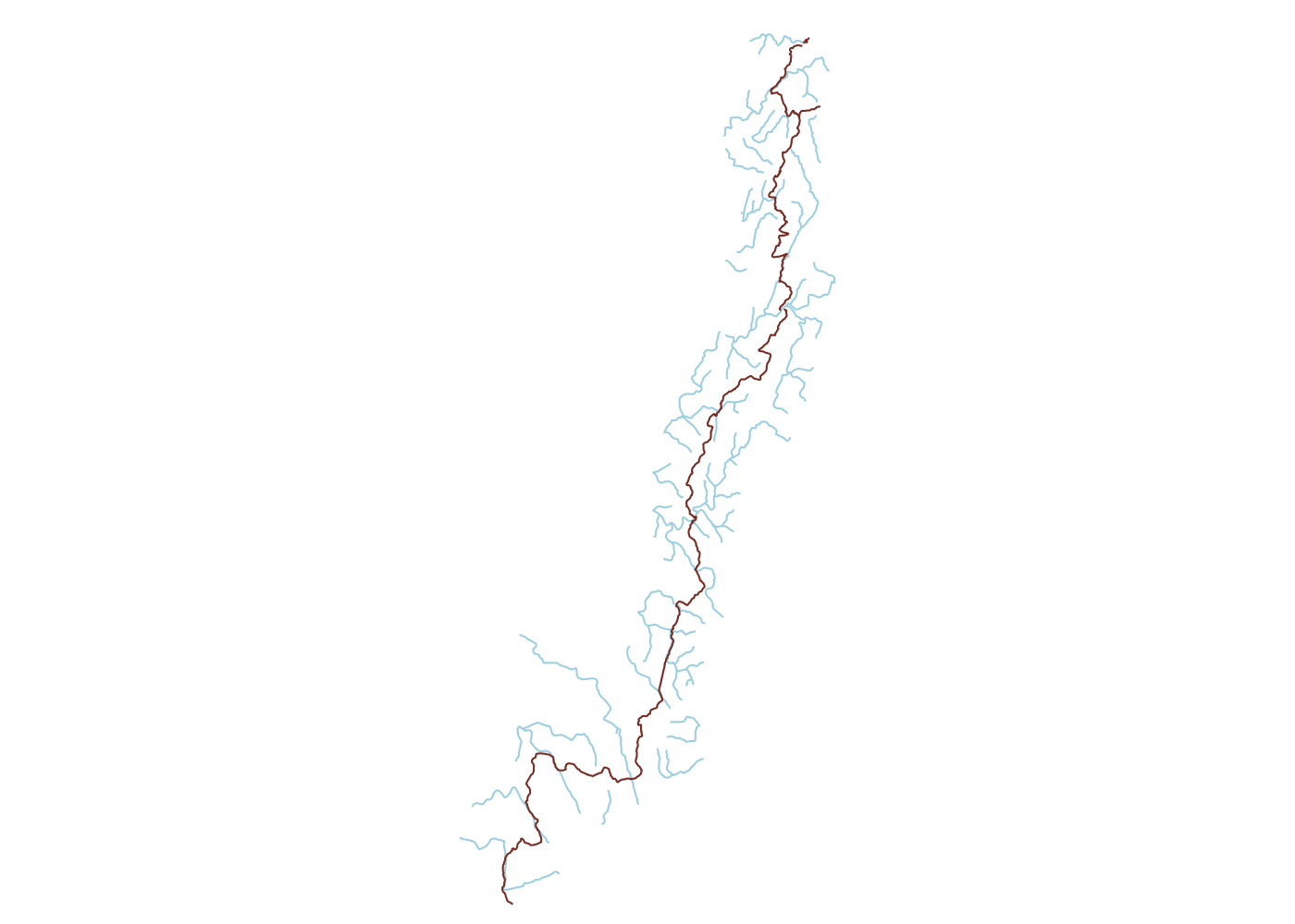
Water
The first other feature we need is water. On any multi-day trip, being able to refill your water is essential. The OSM wiki page on waterways shows us that they values we need to grab relevant water sources are river and stream. Although not well-documented, you can supply multiple value arguments to osmdata::opq() using c(). This will let us quickly and easily grab both rivers and streams in the area.2
## create bbox for just the Uwharrie Trail; no need for all water in the whole National Forest
ut_bb <- matrix(st_bbox(ut), ncol = 2, dimnames = list(c('x', 'y'), c('min', 'max')))

## get rivers and streams and extract OSM lines
ut_water <- opq(bbox = ut_bb) %>%
  add_osm_feature(key = 'waterway', value = c('river', 'stream')) %>%
  osmdata_sf()
Our next step will be to drop any water sources more than a kilometer from the trail. This will simplify our analysis later and also minimizes our environmental impact. To conduct GIS operations in meters, we need to project our data from latitude and longitude-based WGS84 to a meter-based coordiante reference system (CRS). The CRS database epsg.io shows that NAD83/North Carolina(EPSG:32119) is the projection for data in North Carolina, so we use sf::st_transform() along with sf::st_crs() to project our trail and water source objects. This lets us calculate distances in feet/meters rather than decimal degrees. We’ll use this to limit the water features to those that fall within 1km of the trail. This way we’re not limiting ourselves to only water features that directly intersect the trail, but we’re also not retaining a bunch of features that are farther off-trail than I like to hike for water.
## project trail
ut <- st_transform(ut, st_crs(32119))

## project water sources
ut_water <- ut_water$osm_lines %>%
  st_transform(st_crs(32119)) %>%
  st_filter(ut, .predicate = st_is_within_distance, dist = 1000)

## plot
plot(ut_water$geometry, col = 'lightblue')
plot(ut$geometry, add = T, col = 'coral4')
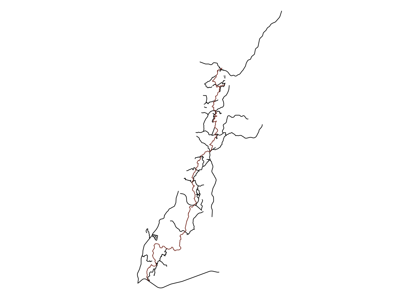
Roads
If we want to be near water, we want to be far from roads. OpenStreetMap has lots of different categories of roads, so we’ll want to capture all the major ones, as well as service roads and “tracks”, which is how OpenStreetMap refers to forest roads.3 OSM identifies roads with the key “highway,” and inspecting the OSM wiki page on roads shows us the various values we’ll need to grab all relevant roads.
## get roads, project, and limit to w/in 1000 m of trail
ut_roads <- opq(bbox = ut_bb) %>%
  add_osm_feature(key = 'highway',
                  value = c('primary', 'secondary', 'tertiary', 'residential',
                            'unclassified', 'track', 'service')) %>%
  osmdata_sf() %>%
  magrittr::extract2('osm_lines') %>%
  st_transform(st_crs(32119)) %>%
  st_filter(ut, .predicate = st_is_within_distance, dist = 1000)

## plot
plot(ut_roads$geometry, col = 'black')
plot(ut$geometry, add = T, col = 'coral4')
Note the use of magrittr::extract2() to extract the osm_lines object from the osmdata_sf object returned by osmdata::osmdata_sf(). This is how you can access a list element in a pipeline, and is equivalent to $osm_lines.
Campsites
To locate potential campsites we need to identify our priorities and use them to define a set of rules for selecting potential sites. For this exercise, I’m using the following:
I’d like to be within 750 feet of a water source. Some (more hardcore) backpackers prefer to be farther away from water sources to minimize the chance of encountering animals. Since Uwharrie National Forest isn’t an area with heightened bear activity, I’m willing to trade the chance of a raccoon sniffing around my bear canister for a shorter walk to refill my water.
The US Forest Service requires that you camp at least 200 feet away from any water source. This is good practice everywhere, but it’s required in National Forests, so we want to make sure any potential campsites are at least 200 feet from any water features.
The Uwharrie Trail is a fairly heavily-trafficked trail, so I’d like to avoid going more than 1/4 mile off-trail to find a campsite. This will minimize the disturbance to the surrounding area.4 All of the semi-official campsites on the Uwharrie Trail are a good ways off the trail itself, so staying near the trail will contain my impact on a large scale, but minimize it locally.
If you’re not in a designated campsite, you should be at least 200 feet away from any trail. Again, this seeks to minimize your impact on the area by spreading out campsites over time.
If I’m making the effort to carry my shelter, sleep system, and food on my back, you better believe I don’t want to be hearing any cars at night. To try and minimize the chances of this happening, I want to be least 1,000 feet from any roads. The lower section of the trail skirts particularly close to a residential neighborhood, so this is an important consideration.
I’m going to drop any potential campsites smaller than 0.1 km^2. Choosing where to actually pitch your tent within a potential site area requires many considerations like drainage, wind exposure, and avoiding dead trees overhead. This means that we want to have ample space in which to find the ideal tent spot, so dropping small potential sites reduces the possibility of arriving at a spot and finding that there’s no good place for your tent.
With all of those factors in mind, we can now define our potential campsites and then narrow them down. I start by buffering the rivers and streams by 1,000 feet with sf::st_buffer(), which gives us every area within 1,000 feet of a water source. Then I move down my list of conditions, buffering the relevant feature and using sf::st_intersect() when I want to ensure I stay within a given distance of that feature and sf::st_difference() when I want to stay a given distance away from that feature.
Since NAD83 uses meters as the unit of measurement, we need to convert these distances in feet into meters. Again, the units package makes this easy with the units::set_units() function.
## buffer water 750 ft
campsites <- st_union(ut_water) %>%
  st_buffer(dist = units::set_units(750, ft))

## buffer water 200 ft and subtract
campsites <- st_union(ut_water) %>%
  st_buffer(dist = units::set_units(200, ft)) %>%
  st_difference(x = campsites)

## buffer trail 1/4 mile and intersect
campsites <- st_union(ut) %>%
  st_buffer(dist = units::set_units(.25, mi)) %>%
  st_intersection(x = campsites)

## buffer trail 200 ft and subtract
campsites <- st_union(ut) %>%
  st_buffer(dist = units::set_units(200, ft)) %>%
  st_difference(x = campsites)

## buffer roads to 1000 ft and subtract
campsites <- st_union(ut_roads) %>%
  st_buffer(dist = units::set_units(1000, ft)) %>%
  st_difference(x = campsites)

## cast multipolygon to polygons and convert to sf
campsites <- campsites %>%
  st_cast('POLYGON') %>%
  st_sf() %>%
  mutate(id = 1:n()) %>% # create ID variable
  filter(st_area(.) > units::set_units(.1, km^2)) # filter to > .1 sq km
The animation below shows each step in the process in order:
Elevation
So far we haven’t really done anything that you couldn’t do on CalTopo, albeit in a less programmatic way. Let’s change that by bringing in some elevation data. Elevation is important when hiking because it determines how many climbs your lungs will have to endure and how many descents your knees will. CalTopo has great built-in tools for generating elevation profiles and more detailed terrain statistics that can tell you what to expect along a given route. However, you can only calculate them for lines or polygons you’ve manually drawn.
While we could import the potential campsite polygons we’ve just generated into CalTopo and then calculate the terrain statistics, this has two major drawbacks. First, you have to point and click through generating the report for each polygon because there’s no way to batch process. Second, and more importantly, this would use a lot of processing power and computing time on CalTopo’s servers. If, unlike me, you have a paid subscription, you might feel less bad about this, but I’m trying not to take advantage of such an awesome service that CalTopo currently provides for free.
We can use R’s capabilities to handle raster data to solve both of these problems! The elevatr package lets you easily download elevation data in the form of a digital elevation model. These models combine multiple measurements from satellites to produce a single image of the earth where the brightness of each pixel represents the elevation of a given area. elevatr allows you to easily access elevation data compiled from a number of different data sources. The main function is elevatr::get_elev_raster(), which takes an sf object as its first argument and z, z zoom level of 1:14. We can also specify the clip = 'bbox' argument to crop the resulting raster to just the bounding box of our potential campsites, and not the entire tile they fall in.
library(raster)
library(elevatr)

## get elevation raster and clip to bbox
elev <- get_elev_raster(campsites, z = 13, clip = 'bbox')

## plot to inspect
plot(elev, col = grey(1:100/100))
plot(ut$geometry, add = T, col = 'coral4')
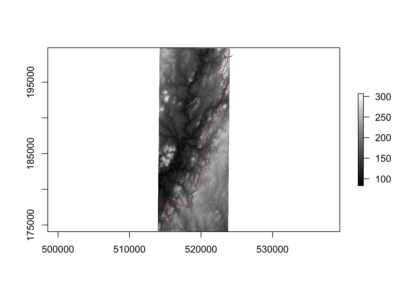
Since we can see that the highest point in the area is only about 300 feet above sea level, we don’t need to worry about absolute elevation when picking potential sites. Instead, we want to know how level these areas are; no one wants to wake up smushed against the downhill wall of their tent. We can use the raster::terrain() function to calculate the slope in each pixel.
## calculate slope
camp_slope <- terrain(elev, opt = 'slope', unit = 'degrees')

## plot slope
plot(camp_slope)
plot(ut$geometry, add = T, col = 'coral4')
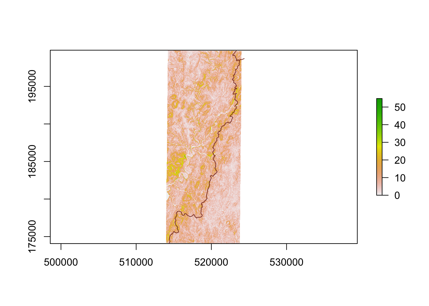
All that’s left to do is aggregate slope measures to each polygon, and then calculate some sort of summary statistic to tell us how steep each potential site is overall. I’m going to use the median of each area’s slope rather than its average to avoid giving undue influence to outliers (if a .5 km2 area is largely flat with a cliff at one edge, then it’s likely still a good candidate for a campsite). Let’s filter out all areas with a median slope of more than 10°.
## calculate median slope for each polygon and filter
campsites <- campsites %>%
  mutate(med_slope = (raster::extract(camp_slope, ., fun = median, na.rm = T))) %>%
  filter(med_slope < 10)
With that done, we can now plot our potential campsite locations and all the features used to define them:
## plot campsites and all features
plot(ut$geometry, type = 'n')
plot(campsites$geometry, add = T, col = 'lightgreen', border = NA)
plot(ut_water$geometry, add = T, col = 'lightblue')
plot(ut_roads$geometry, add = T, col = 'black')
plot(ut$geometry, add = T, col = 'coral4')
This is a pretty picture, but it’s not very useful. To make it so that we can actually navigate to any of these spots, we need to get them onto a topographic map.
Plan it
To make our map usable, all we have to do is export the potential campsite polygons from R so that we can import them into CalTopo. CalTopo supports a number of file formats for importing, but the one we want to use is GeoJSON. We can use the geojsonio package to easily convert our polygons from sf objects to GeoJSON format and then save them to disk to import into CalTopo.5
There are two (potentially) tricky things we need to do. First, make sure we reproject our NAD83 data back to decimal degree-based WGS84 so that CalTopo can properly reference them. Second, we want to take advantage of R’s capabilities to efficiently wrangle data and create a name field for our polygons so they’ll be easy to identify and reference once they’re in CalTopo. To do this, we need to create a “title” field in our sf object before we convert it to GeoJSON.6
library(geojsonio)

## create site number field; transmute b/c all fields other than label are lost on import
campsites %>%
  transmute(title = str_c('Potential Site ', row_number())) %>%
  st_transform(st_crs(4326)) %>% # project to WGS84
  geojson_json() %>%
  geojson_write(file = 'campsites.json')

## export Uwharrie Trail to save the trouble of tracing it
ut %>%
  st_transform(st_crs(4326)) %>% # project to WGS84
  geojson_json() %>%
  geojson_write(file = 'trail.json')
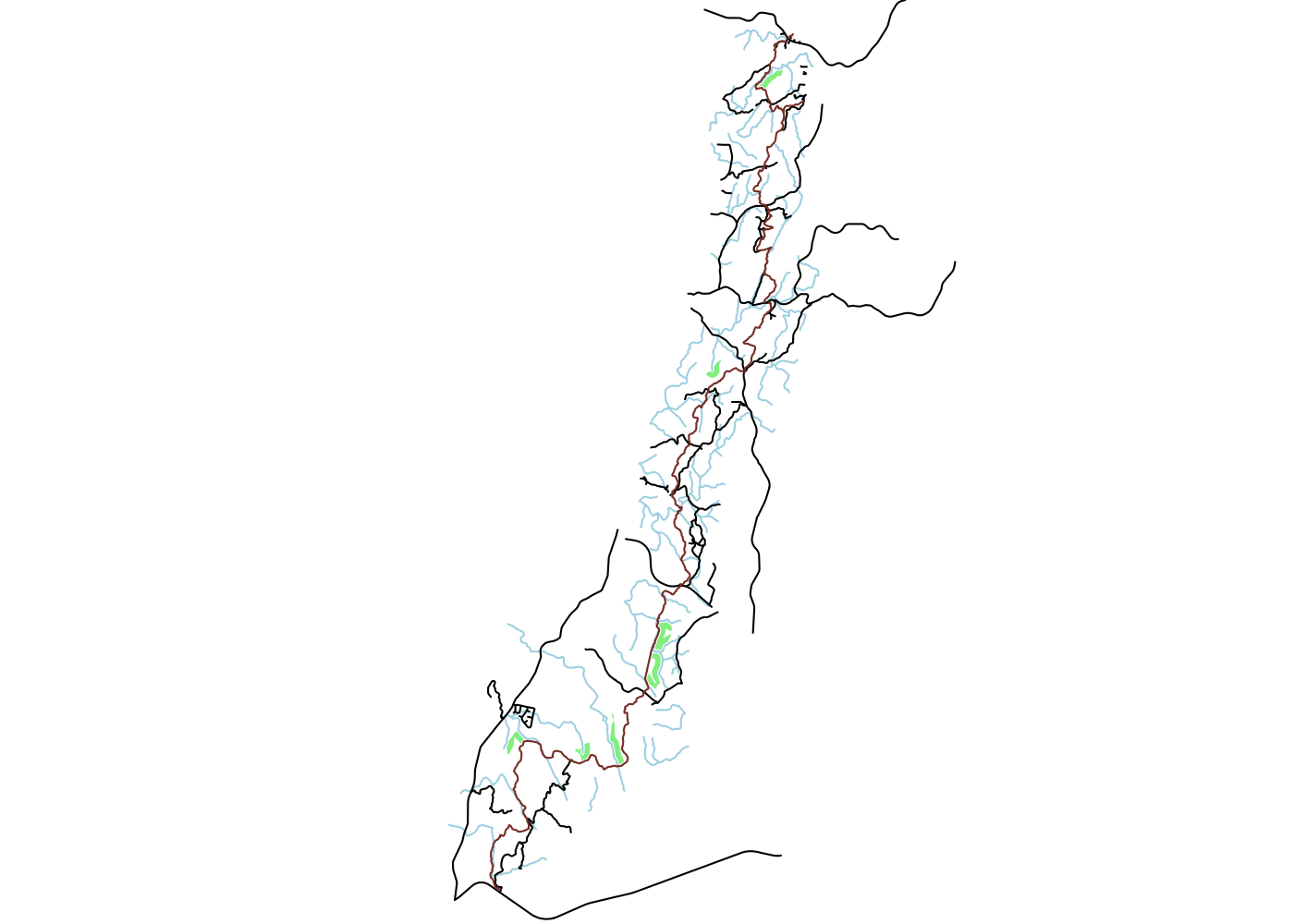
At this point all that’s left to do is click the “Import” button in CalTopo and select your newly created .json file. You can check out the potential campsites live on CalTopo below:
Some closing thoughts viewing the potential sites in context on CalTopo:
- Potential Site 2 looks promising. It’s slightly downhill from the trail, and has some relatively flat ground. However, the water source is an intermittent stream (denoted by the three dots in the blue line), so depending on time of year there may not actually be easy access to water here.
- Potential Site 4 is located near both a perennial and an intermittent stream, so the odds of finding a usable water source are higher. Across the trail to the West you can see an area that meets all of our site selection criteria except gentle slopes due to the steep rise to the 795 foot peak nearby.
- Potential Site 7 demonstrates the limitations of this approach because there are two forest roads near it on the Forest Service map that aren’t included in OpenStreetMap. Google Maps shows that there’s a private RV campground here, so best to avoid it. Doubly so because it’s largely outside of Uwharrie National Forest’s boundaries (the green lines). This is why it’s important to check more than just the terrain before you go!
See here for a discussion of different types of campsites and contexts in which they are usually found. ↩
If we didn’t do this, we’d have to use
c()to combine multipleosmdata_sfobjects and then extract theosm_linesobject from the combinedosmdata_sfobject. ↩The US Forest Service maintains GIS data on forest roads on National Forest land, but the API to access them is…less than user friendly so I’m ignoring them for this illustration. ↩
In very sparsely-traveled areas, it can be better to seek out campsites far from the trail to avoid camping in areas where others have recently stayed. This can help prevent the emergence of ‘social’ campsites that are not officially recognized or maintained but are frequently used. It will also reduce the chance that you’ll encounter any local wildlife that have learned that such spots can be a source of easy meals. ↩
Want to find potential campsites for a trail that’s not in OpenStreetMap? CalTopo supports exports as well as imports, so you can trace the route in CalTopo, export it, then load it in R with
sf::st_read()and then carry out the steps above! ↩CalTopo refers to an object’s name field as its “Label” in the interface, but this isn’t what it’s called under the hood. I had to export a line I create and inspect the resulting
.jsonfile to find out that it’s referred to as a “title” instead. ↩