
Extracting UN Peacekeeping Data from PDF Files
Published:
Some coauthors and I recently published a piece in the Monkey Cage on the recent military coup in Mali and the overthrow of president Ibrahim Boubacar Keïta. We examine what the ouster of Keïta means for the future of MINUSMA, the United Nations peacekeeping mission in Mali. One of my contributions that didn’t make the final cut was this plot of casualties to date among UN peacekeepers in the so-called big 5 peacekeeping missions .
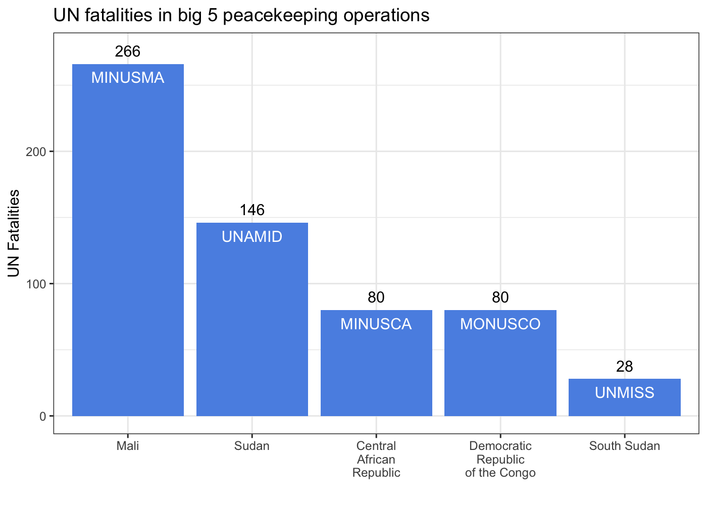
These missions are distinguished from other current UN peacekeeping missions by high levels of violence (both overall and against UN personnel) and expansive mandates that go beyond ‘traditional’ goals of stabilizing post-conflict peace. The conflict management aims of these operations necessarily expose peacekeepers to high levels of risk. If we want to try understand what the future of MINUSMA might look like dealing with a new government in Mali, it’s important to place MINUSMA in context among the remainder of the big 5 missions. To help do so, I turned to the source for data on peacekeeping missions, the UN.
Nonstandard formats
When we wrote the piece, the Peacekeeping open data portal page on fatalities only had a link to this PDF report instead of the usual CSV file (the CSV file is back, so you don’t technically have to go through all of these steps to recreate this figure). Here’s what the first page of that PDF looks like:
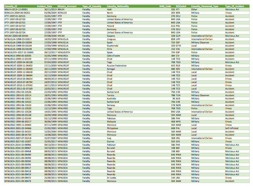 Since we were working on a short deadline, I needed to get these data out of that PDF. The most direct option is to just copy and paste the data into an Excel sheet. However, these data run to 148 pages, so all that copying and pasting would be tiring and risks introducing errors when your attention eventually slips and you forget to include page 127.
Getting the data
Enter the tabulizer R package. This package is just a (much) friendlier wrapper to the Tabula Java library, which is designed to extract tables from PDF documents. To do so, just plug in the file name of the local PDF you want or URL for a remote one:
library(tabulizer)

## data PDF URL
dat <- 'https://peacekeeping.un.org/sites/default/files/fatalities_june_2020.pdf'

## get tables from PDF
pko_fatalities <- extract_tables(dat, method = 'stream')
The extract_tables() function has two different methods for extracting data: lattice for more structured, spreadsheet like PDFs and stream for messier files. While the PDF looks pretty structured to me, method = 'lattice' returned a series of one variable per line gibberish, so I specify method = 'stream' to speed up the process by not forcing tabulizer to determine which algorithm to use on each page.
Note that you may end up getting several warnings, such as the ones I received:
## WARNING: An illegal reflective access operation has occurred
## WARNING: Illegal reflective access by RJavaTools to method java.util.ArrayList$Itr.hasNext()
## WARNING: Please consider reporting this to the maintainers of RJavaTools
## WARNING: Use --illegal-access=warn to enable warnings of further illegal reflective access operations
## WARNING: All illegal access operations will be denied in a future release
Everything still worked out fine for me, but you may run into problems in the future based on the warning about future releases.
Cleaning the data
We end up with a list that is 148 elements long, one per page. Each element is a matrix, reflecting the structured nature of the data. Normally, we could just combine this list of matrices into a single object with do.call(rbind, pko_fatalities):
do.call(rbind, pko_fatalities)
## Error in (function (..., deparse.level = 1) : number of columns of matrices must match (see arg 2)
But if we do this, we get an error! Let’s take a look and see what’s going wrong. We can use lapply() in combination with dim() to do so:
head(lapply(pko_fatalities, dim))
## [[1]]
## [1] 54  9
##
## [[2]]
## [1] 54  7
##
## [[3]]
## [1] 54  7
##
## [[4]]
## [1] 54  7
##
## [[5]]
## [1] 54  7
##
## [[6]]
## [1] 54  7
The first matrix has an extra two columns, causing our attempt to rbind() them all together to fail.
head(pko_fatalities[[1]])
##      [,1]                   [,2]                            [,3] [,4]
## [1,] "Casualty_ID"          "Incident_Date Mission_Acronym" ""   "Type_of_Casualty"
## [2,] "BINUH‐2019‐12‐00001"  "30/11/2019 BINUH"              ""   "Fatality"
## [3,] "BONUCA‐2004‐06‐04251" "01/06/2004 BONUCA"             ""   "Fatality"
## [4,] "IPTF‐1997‐01‐02515"   "31/01/1997 IPTF"               ""   "Fatality"
## [5,] "IPTF‐1997‐09‐02720"   "17/09/1997 IPTF"               ""   "Fatality"
## [6,] "IPTF‐1997‐09‐02721"   "17/09/1997 IPTF"               ""   "Fatality"
##      [,5]                       [,6]                [,7] [,8]
## [1,] "Casualty_Nationality"     "M49_Code ISOCode3" ""   "Casualty_Personnel_Type"
## [2,] "Haiti"                    "332 HTI"           ""   "Other"
## [3,] "Benin"                    "204 BEN"           ""   "Military"
## [4,] "Germany"                  "276 DEU"           ""   "Police"
## [5,] "United States of America" "840 USA"           ""   "Police"
## [6,] "United States of America" "840 USA"           ""   "Police"
##      [,9]
## [1,] "Type_Of_Incident"
## [2,] "Malicious Act"
## [3,] "Illness"
## [4,] "Accident"
## [5,] "Accident"
## [6,] "Accident"
head(pko_fatalities[[2]])
##      [,1]                    [,2]                 [,3]       [,4]       [,5]
## [1,] "MINUSCA‐2015‐10‐09459" "06/10/2015 MINUSCA" "Fatality" "Burundi"  "108 BDI"
## [2,] "MINUSCA‐2015‐10‐09468" "13/10/2015 MINUSCA" "Fatality" "Burundi"  "108 BDI"
## [3,] "MINUSCA‐2015‐11‐09509" "10/11/2015 MINUSCA" "Fatality" "Cameroon" "120 CMR"
## [4,] "MINUSCA‐2015‐11‐09510" "22/11/2015 MINUSCA" "Fatality" "Rwanda"   "646 RWA"
## [5,] "MINUSCA‐2015‐11‐09511" "30/11/2015 MINUSCA" "Fatality" "Cameroon" "120 CMR"
## [6,] "MINUSCA‐2015‐12‐09542" "06/12/2015 MINUSCA" "Fatality" "Congo"    "178 COG"
##      [,6]                     [,7]
## [1,] "Military"               "Malicious Act"
## [2,] "Military"               "Accident"
## [3,] "Military"               "Malicious Act"
## [4,] "Military"               "To Be Determined"
## [5,] "International Civilian" "Illness"
## [6,] "Military"               "Illness"
We can see that the first page has two blank columns, accounting for the 9 columns compared to the 7 columns for all other pages. Closer inspection of the header on the first page and the columns on both the first and second pages reveals that there actually should be 9 columns in the data.
The Incident_Date and Mission_Acronym columns are combined into one, as are the M49_Code and ISOCode3 columns. We’ll fix the data in those two columns in a bit, but first we have to get rid of the empty columns in the first page before we can merge the data from all the pages. We could just tell R to drop those columns manually with pko_fatalities[[1]][, -c(3, 7)], but this isn’t a very scalable solution if we have lots of columns with this issue.
To do this programmatically, we need a way to identify empty columns. If this was a list of data frames, we could use colnames() to identify the empty columns. However, extract_tables() has given us a matrix with the column names in the first row. Instead, we’ll just get the first row of the matrix. Since we’re accessing a matrix that is the first element in a list, we want to use pko_fatalities[[1]][1,] to index pko_fatalities. Next, we’ll use the grepl() function to identify the empty columns. We want to search for the regular expression ^$, which means the start of a line immediately followed by the end of a line, i.e., an empty string. Finally, we negate it with a ! to return only non-empty column names:
## drop two false empty columns on first page
pko_fatalities[[1]] <- pko_fatalities[[1]][, !grepl('^$', pko_fatalities[[1]][1,])]
With that out of the way, we can now combine all the pages into one giant matrix. After that, I convert the matrix into a data frame, set the first row as the column names, and then drop the first row.
## rbind pages
pko_fatalities <- do.call(rbind, pko_fatalities)

## set first row as column names and drop
pko_fatalities <- data.frame(pko_fatalities)
colnames(pko_fatalities) <- (pko_fatalities[1, ])
pko_fatalities <- pko_fatalities[-1, ]
Now that we’re working with a data frame, we can finally tackle those two sets of mashed up columns. To do this, we’ll use the separate() function in the dplyr package, which I load via the tidyverse package. Separate is magically straightforward. It takes a column name (which I have to enclose in backticks thanks to the space), a character vector of names for the resulting columns, and a regular expression to split on. I use \\s, which matches any whitespace characters. I also filter out any duplicate header rows that may have crept in (there’s one on page 74, at the very least).
library(tidyverse)

## separate columns tabulizer incorrectly merged
pko_fatalities <- pko_fatalities %>%
  filter(Casualty_ID != 'Casualty_ID') %>% # drop any repeated header(s)
  separate(`Incident_Date Mission_Acronym`, c('Incident_Date', 'Mission_Acronym'),
           sep = '\\s', convert = T, extra = 'merge')  %>%
  separate(`M49_Code ISOCode3`, c('M49_Code', 'ISOCode3'),
           sep = '\\s', convert = T) %>%
  mutate(Incident_Date = dmy(Incident_Date)) # convert date to date object
You’ll notice I also supply two other arguments here: convert and extra. The former will automatically convert the data type of resulting columns, which is useful because it converts Incident_Date into a Date object, and M49_Code into an int object. The latter tells separate() what to do if it detects more matches of the splitting expression than you’ve supplied column names. There are 18 observations where the mission acronym is list as “UN Secretariat”. That means that separate() will detect a second whitespace character in these 18 rows. If you don’t explicitly set extra, you’ll get a warning telling you what happened with those extra characters. By setting extra = 'merge', you’re telling separate() to effectively ignore any space after the first one and keep everything to the right of the first space as part of the output. Thus, our "UN Secretariat" observations are preserved instead of being chopped off to just "UN".
Creating the plot
Now that we’ve got the data imported and cleaned up, we can recreate the plot from the Monkey Cage piece. However, first we need to bring in some outside information and calculate some simple statistics.
Preparing the data
Before we can plot the data, we need to bring in some mission-level information, namely what country each mission operates in. We can get this easily from the Peacekeeping open data portal master dataset. Once I load the data into R I select just the mission acronym and country of operation. I then edit the strings for CAR and DRC to add newlines between words with \n to make them fit better into the plot.
## get active PKO data and clean up country names
read_csv('https://data.humdata.org/dataset/819dce10-ac8a-4960-8756-856a9f72d820/resource/7f738eb4-6f77-4b5c-905a-ed6d45cc5515/download/coredata_activepkomissions.csv') %>%
  select(Mission_Acronym, Country = ACLED_Country) %>%
  mutate(Country = case_when(Country == 'Central African Republic' ~
                               'Central\nAfrican\nRepublic',
                             Country == 'Democratic Republic of Congo' ~
                               'Democratic\nRepublic\nof the Congo',
                             TRUE ~ Country)) -> pko_data
We’re looking to see how dangerous peacekeeping missions are for peacekeepers, so we want to only look at fatalities that are the result of deliberate acts. The data contain 6 different types of incident, so let’s check them out:
table(pko_fatalities$Type_Of_Incident)
##
##         Accident          Illness    Malicious Act   Self‐Inflicted To Be Determined
##             2712             2582             2096              268              244
##          Unknown
##               50
Malicious acts are the third highest type of incident, so it’s important for us to subset the data to ensure we’re counting the types of attacks we’re interested in. Since we’re looking at fatalities in the big 5 missions, we also need to subset the data to just these missions. We’re going to use the summarize() function in conjunction with group_by() to calculate several summary statistics for each mission. We’ll also use the time_length() and interval() functions from the lubridate package, so load that as well.
library(lubridate)

## list of PKOs to include
pkos <- c('MINUSMA', 'UNAMID', 'MINUSCA', 'MONUSCO', 'UNMISS')

## aggregate mission level data
pko_fatalities %>%
  filter(Type_Of_Incident == 'Malicious Act',
         Mission_Acronym %in% pkos) %>%
  group_by(Mission_Acronym) %>%
  summarize(casualties = n(),
            casualties_mil = sum(Casualty_Personnel_Type == 'Military'),
            casualties_pol = sum(Casualty_Personnel_Type == 'Police'),
            casualties_obs = sum(Casualty_Personnel_Type == 'Military Observer'),
            casualties_civ = sum(Casualty_Personnel_Type == 'International Civilian'),
            casualties_oth = sum(Casualty_Personnel_Type == 'Other'),
            casualties_loc = sum(Casualty_Personnel_Type == 'Local'),
            duration = time_length(interval(min(Incident_Date),
                                            max(Incident_Date)),
                                   unit = 'year')) %>%
  mutate(MINUSMA = case_when(Mission_Acronym == 'MINUSMA' ~ 'MINUSMA',
                             TRUE                         ~ '')) %>%
  left_join(pko_data, by = 'Mission_Acronym') %>%
  mutate(Country = factor(Country,
                          levels = Country[order(casualties,
                                                 decreasing = T)])) -> data_agg
casualties = n()counts the total number of fatalities in each mission because each row is one fatalitycasualties_mil = sum(Casualty_Personnel_Type == 'Military')counts how many of those casualties were UN troops- the other
casualties_...lines do the same for different categories of UN personnel - the code to the right of
durationcalculates how long each mission has lasted by:- finding the first and last date of a fatality in each mission
- creating an
intervalobject from those dates - calculating the length of that period in years
- create an indicator variable noting whether or not an observation belongs to MINUSMA
Finally, we merge on the country information contained in pko_data and convert Country to a factor with levels that are decreasing in fatalities. This last step is necessary to have a nice ordered plot.
Plot it
With that taken care of, we can create the plot using ggplot. I’m using the label argument to place mission acronyms inside the bars with geom_text(), and a second call to geom_text() with the casualties variable to place fatality numbers above the bars. The nudge_y argument in each call to geom_text() ensures that they’re vertically spaced out, making them readable instead of overlapping.
ggplot(data_agg, aes(x = Country, y = casualties, label = Mission_Acronym)) +
  geom_bar(stat = 'identity', fill = '#5b92e5') +
  geom_text(color = 'white', nudge_y = -10) +
  geom_text(aes(x = Country, y = casualties, label = casualties),
            data = data_agg, inherit.aes = F,
            nudge_y = 10) +
  labs(x = '', y = 'UN Fatalities',
       title = 'UN fatalities in big 5 peacekeeping operations') +
  theme_bw()
Plot it (again)
We can also create some other plots to visualize how dangerous each mission is to peacekeeping personnel. While total fatalities are an important piece of information, the rate of fatalities can tell use more about the intensity of the danger in a given conflict.
data_agg %>%
  ggplot(aes(x = duration, y = casualties, label = MINUSMA)) +
  geom_point(size = 2.5, color = '#5b92e5') +
  geom_text(nudge_x = 1) +
  expand_limits(x = 0, y = 0) +
  labs(x = 'Mission duration (years)', y = 'Fatalities (total)',
       title = 'UN fatalities in big 5 peacekeeping operations') +
  theme_bw()
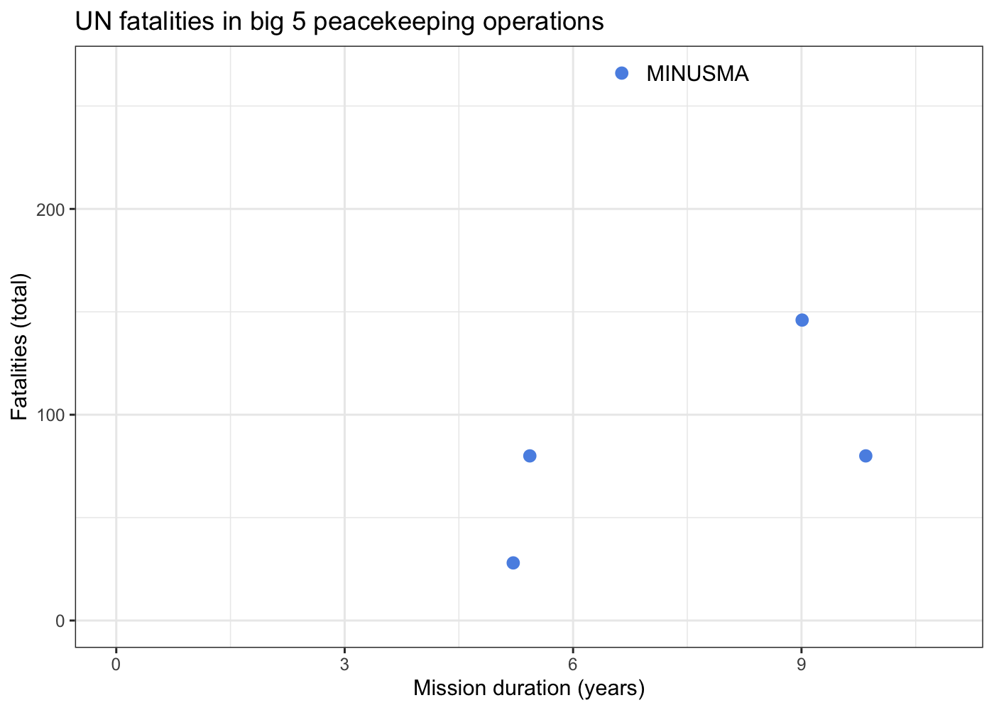
We can see from this plot that not only does MINUSMA have the most peacekeeper fatalities out of any mission, it reached that point in a comparatively short amount of time. To really drive this point home, we can draw on the fantastic gganimate package. We’re going to animate cumulative fatality totals over time, so we need a yearly version of our mission-level data frame from above. The code below is pretty similar except we’re grouping by both Mission_Acronym and a variable called Year what we’re generating with the year() function in lubridate (it extracts the year from a Date object).
pko_fatalities %>%
  filter(Type_Of_Incident == 'Malicious Act',
         Mission_Acronym %in% pkos) %>%
  group_by(Mission_Acronym, Year = year(Incident_Date)) %>%
  summarize(casualties = n(),
            casualties_mil = sum(Casualty_Personnel_Type == 'Military'),
            casualties_pol = sum(Casualty_Personnel_Type == 'Police'),
            casualties_obs = sum(Casualty_Personnel_Type == 'Military Observer'),
            casualties_civ = sum(Casualty_Personnel_Type == 'International Civilian'),
            casualties_oth = sum(Casualty_Personnel_Type == 'Other'),
            casualties_loc = sum(Casualty_Personnel_Type == 'Local')) %>%
  mutate(MINUSMA = case_when(Mission_Acronym == 'MINUSMA' ~ 'MINUSMA',
                             TRUE                         ~ ''),
         Mission_Year = Year - min(Year) + 1) %>%
  left_join(pko_data, by = 'Mission_Acronym') %>%
  mutate(Country = factor(Country, levels = levels(data_agg$Country))) -> data_yr
Once we’ve done that, we need to make a couple tweaks to our data to ensure that our plot animates correctly. I use the new across() function (which is likely going to eventually replace mutate_at, mutate_if, and similar functions) to select all columns that start with “casualties”. Then, I supply the cumsum() function to the .fns argument, and use the .names argument to append “_cml” to the end of each resulting variable’s name. This argument uses glue syntax, which allows you to embed R code in strings by enclosing it in curly braces. The complete() function uses the full_seq() function to fill in any missing years in each mission, i.e., a year in the middle of a mission without any fatalities due to malicious acts. Finally, the fill() function fills in any rows we just added that are missing fatality data due to an absence of fatalities that year.
Now we’re ready to animate our plot! We construct the ggplot object like before, but this time we add the transition_manual() function to the end of the plot specification. This function tells gganimate what the ‘steps’ in our animation are. Since we’ve got individual years, we’re using the manual version of transition_ instead of the many fancier versions included in the package.
If you check out the documentation for transition_manual(), you’ll notice that there are a handful of special label variables you can use when constructing your plot. These will update as the plot cycles through its frames, allowing you to convey information about the flow of time. I’ve used the current_frame variable, again with glue syntax, to make the title of the plot display the current mission year as the frames advance.
library(gganimate)

data_yr %>%
  arrange(Mission_Year) %>%
  mutate(across(starts_with('casualties'), .fns = cumsum, .names = '{col}_cml')) %>%
  complete(Mission_Year = full_seq(Mission_Year, 1)) %>%
  fill(Year:casualties_loc_cml, .direction = 'down') %>%
  filter(Mission_Year <= 6) %>% # youngest mission is UNMISS
  ggplot(aes(x = Country, y = casualties_cml, label = casualties_cml)) +
  geom_bar(stat = 'identity', fill = '#5b92e5') +
  geom_text(nudge_y = 10) +
  labs(x = '', y = 'UN Fatalities',
       title = 'UN fatalities in big 5 peacekeeping operations: mission year {current_frame}') +
  theme_bw() +
  transition_manual(Mission_Year)
While the scatter plot above illustrates that UN personnel working for MINUSMA have suffered the most violence in the shortest time out of any big 5 mission, this animation make it abundantly clear, especially since MONUSCO and UNMISS both experience years without a single UN fatality from a deliberate attack. Visualizations like these are a great way to showcase your work, especially if you’re dealing with dynamic data. While you still can’t easily include them in a journal article, they’re fantastic tools for conference presentations or